Evaluation

The following minimum example serves as a demonstration of the calculation process. The respective sample data sets are RSWA_export_3.json and Destructive_set_3.CSV which are shipped with the software. For the sake of simplicity only one algorithm setting is inspected here.

Measurement Data

At first the absolute adjustment $AA$ is calculated. This is the vertical displacement of the correlation gradient. In order find $AA$ the difference between DT and NDT measurements is calculated. The mean of those differences is the absolute adjustment which minimizes the sum difference between DT and NDT measurements, $-0.19$ in this case.

Calculation

$AA = \frac{1}{N} \sum_i^N D_{DT, i} - d_{NDT, i}$

Point	DT [mm]	NDT [mm]	DT - NDT [mm]	NDT corrected [mm]	| NDT corrected - DT| [mm]	(NDT corrected - DT )² [mm²]
1	0.0	0.00	0.00	-0.19	0.19	0.04
2	1.5	2.75	-1.25	2.56	1.06	1.11
3	4.5	4.47	0.03	4.28	0.22	0.05
4	6.5	6.06	0.44	5.87	0.63	0.40
Mean	3.13	3.32	-0.19	3.12	0.53	0.40

By applying the absolute adjustment a new result vektor for the non-destructive measurements is created, NDT corrected. The mean of this new vector is equal to the mean of the destructive measurements. Thus, both measurements, DT and NDT, have the same extected value, 3.13 here (or 3.12 due to rounding issues). All following steps are based on the corrected NDT values.

Next, the DT measurements are subtracted from the NDT measurements and considered as absolutes. The mean of these values is the mean error per measurement $\overline{\delta_{abs}}$, here $0.53$.

$\overline{\delta_{abs}} = \frac{1}{N} \sum_i^N |d_{NDT, corr, i} - d_{DT, i}|$

In praxis, this is the expected deviation of RSWA measurements with respect to the buttoned out measurements.

For similar algorithm settings its possible that multiple parameter sets yield the same results and consequently the same absolute errors. In this case, the variance of the NDT results should be taken into consideration while choosing the right algorithm setting. Suppose a algorithm setting creates a deviation of half a millimeter for all measurements. This setting would be prefferable in comparison to another which flucutuates between 1 millimeter off and 0. Mathematically this is the error variance $VAR_{\delta}$, the squared difference between NDT and DT measurements.

$VAR_{\delta} =\frac{1}{N} \sum_i^N (d_{NDT, corr, i} - d_{DT, i})^2$

Choosing a fitting Algorithm

With the value pair (error vraiance; mean error) the various algorithm settings can be compared in quality. The ranking list sorts these in order of increasing error variance and secondly with increasing mean error. For a better overview the ranking plot displays those metrics visually (s. User Interface).

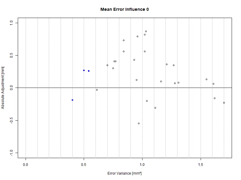
To the left the value pair (0.53; 0.40) can be found, the one just calculated. Generally, the optimization follows the axes -- error variance as well as mean error should go against 0. The more to the left and the vertical center a setting is placed, the better the NDT measurements match the DT reports.

In the plot above, similar to the sample data set, the three algorithm settings furthest to the left are highlighted. Their error variances are 0.40, 0.50, and 0.54. However, it can be seen that a marginally higher error variance of 0.61 would allow for a drastically smaller absolute adjustment. With real, more comprehensive data sets, this effect could be seen more drastically even.

In case the mean error should be given more weight, in the correlation settings the influence of the absolute adjustment may be configured. The plot above displayed used a weight of 0. This implies that the absolute adjustment does not influence the sorting of the algorithm settings. The dashed lines mark areas of equal quality with respect to the ordering.

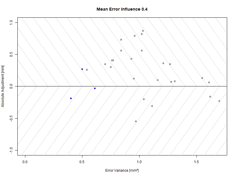
Even with a weight $\alpha$ of 0.4 the forth algorithm at (0.61; -0.33) is now proposed for evaluation. That discards the third point at (0.54; 0.26). The ranking of these algorithms is given by the weighted sum of the error variance and the absolute adjustment $q$.

$q = VAR_{\delta} + \alpha \overline{\delta_{abs}}$

More specifically, this implies the fourth point is given a quality score $q$ of 0.62 while the third point is only 0.64. Since the quality score is minimized, the fourth algorithm is now preferred over the third. This workflow avoids having cscans display vastly different diameters with respect to the actual measurement result.

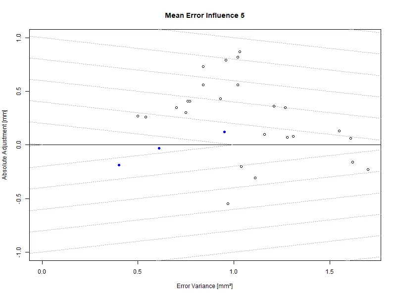
An example for a more conservative setting is the following weight of 5. It can be seen that the equi-quality lines are very steep. This preferres algorithm settings with a low absolute adjustment over anything else, disregarding a higher error variance. The precise setting of this parameter is reliant on the stack thicknesses and the extent of measurement results.

Additional statistical Indicators

Aside from the error variance and the absolute adjustment, other statistical indicators are calculated that are explained below.

Mean Absolute Error

The mean absolute error sums the absolute errors and takes that sum's mean. The difference to the mean error is that positive and negative deviations to not mitigate each other. Instead they sum. It also provides an indication for the mean amount of deviation between DT and NDT.

Regression Line

The graphical comparison of DT and NDT contains a linear regression. This line shows the trend of that scatter plot. Ideally, the linear regression would have a slope of 1, which would imply a 1:1 correlation between NDT and DT.

Coefficient of Determination

The coefficient of determination is a measure for the validity of the linear regression. A coefficient of determination of 1 implies that all points follow the linear trend that is shown by the linear regression. A coefficient of 0 implies that the linear regression is drawn across cluster of seemingly independant points and should not be taken into consideration.

Error Standard Deviation

The error standard deviation is the square root of the error variance. Since many internal guidelines refer to the standard deviation its listed here.

Binary Classification

Calculating a DT-NDT fit is merely the first step in assessing the weld quality. While this relation has to be as close as possible, it is ultimately the match of DT and NDT decisions that are important. In other words, ideally both destructive and ultrasound tests come to the same conclusion for every given weld. In general, there are four scenarios possible;

• good welds that are recognized as good by the RSWA (true positive)
• bad welds that are recognized as good by the RSWA (false positive)
• bad welds that are recognized as bad by the RSWA (true negative)
• good welds that are recognized as bad by the RSWA (false negative)

This might also be structured in a table:

RSWA \ weld quality	ok	not ok
ok	true positive	false positive
not ok	false negative	true negative

There is a caveat; the weld quality cannot be changed. For matching decisions, the assessment of the ultrasound result must be modified. In the RSWA there is a decision diameter that may be different from the decision diameter of destructive testing.

Implementation

In general, all ultrasound results must compare to destructive test results. The criterium for passing or failing a weld is the minimum diameter which is, in turn, related to the plate thickness. The destructive decision threshold is calculated as

$d_{min,DT} = \alpha \sqrt{t_{min}}$

$\alpha$ may be set in Settings→Correlation Settings→Factor $\alpha$ for min. diameter calculation. Most commonly it ranges between 3.5 to 4.025. Next to this setting, the RSWA threshold range for the binary classification may be set as well.

The ultrasound decision threshold follows a similar concept but is, in turn, independent from the destructive decision threshold. Welds that have been failed due to an insufficient destructive diameter may now pass and vice versa. In planning, this can be understood as creating what-if-scenarios. Essentially, how many welds would be rejected/passed if the decision threshold would be at this exact diameter.

By default, the Correlator App plots the decision results as their relative shares over an RSWA decision threshold range of 0 - 12mm, see image below. This plot can be calculated for any given stack thickness combination.

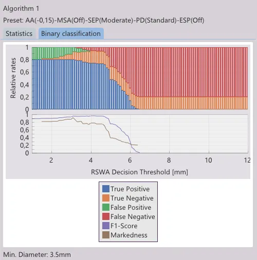
The top half of the plot is the classification over diameter mentioned above. Those four decision outcomes are encoded by color. Their visibility can be toggled by clicking on the respective entry in the legend.

In the bottom half are performance indicators. The F1-score shows the relation of true positives to true positives, false positives and false negatives. If this value approaches 1, the amount of false decisions by the RSWA are minimized. If the F1-score approaches 0, it means that all decisions are false. Markedness, on the other hand, is an indicator that sums positive and negative predictive values. Those are true positives over predicted positives and true negatives over predicted negatives. It also ranges between 0 and 1, with 1 being the desirable outcome. Further reading on wikipedia.

Generally one should be interested in maximizing the accuracy, that is (true positive + true negative) in relation to the entire population. It can be visualized by looking at the stacked columns of blue and yellow. Ideally, this ratio is 1, meaning all decisions of the RSWA correspond to the findings of destructive testing. In reality, and especially for bigger data sets, there will be non-matching decisions.

There is a strong bias towards false negative compared to false positive, as in the former case parts may be scrapped in error, whereas in the latter case bad quality parts slip through undetected. Most likely this is to be avoided, however compromises have to be made. This may be illustrated with an example.

Example

The picture above shows a good to bad weld ratio of about 4 to 1, as indicated by the ratios of the colored bars on the extreme left and right hand side of the plot. Welds are ranging between 1 and 6 millimeter with the majority of about 5 millimeter, since there are the most prominent changes in colored bar gradients.

At first, one would look for a diameter range where F1-score, markedness, and accuracy, that is true positive and true negative, are maximized. In the example above it would yield in a range of about 3.5 to 4.5 millimeter. Next would be an avoidance of false positive results, meaning the abscence of the green area. It can be seen that from decision diameters exceeding 4.0 millimeter, no false positives can be found. Hence, the resulting range is narrowed to to an interval between 4.0 and 4.5 millimeter. To account for measurement uncertainty and repeatability and also considering the steep decline in detection rate at about 5 millimeter, it is advisable to set the decision diameter for that plate combination to about 4.3 millimeter. It can be seen that the detection rate is at about 93 percent and all misclassifications were false negative, meaning all bad welds were successfully detected.